2. Using KAT
KAT is a C++ program containing a number of subtools which can be used in
isolation or as part of a pipeline. Typing kat --help will show a
list of the available subtools. Each subtool has its own help system which you
can access by typing kat <subtool> --help.
2.1. HIST
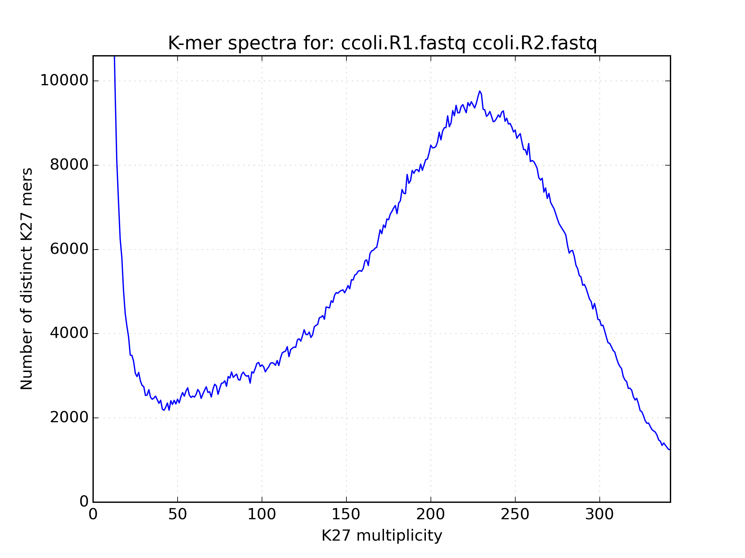
Creates a histogram with the number of distinct k-mers having a given frequency, derived from the input. The input can take the form of one or more FastA or FastQ files, or a jellyfish hash. The last bucket in the histogram behaves as a catchall: it tallies all k-mers with a count greater or equal to the low end point of this bucket.
This tool is very similar to the histo tool in jellyfish itself. The primary
difference being that the output contains metadata that make the histogram easier
for the user to plot, and that this version is faster because we do not need to
dump the hash to disk and read it back.
Basic usage:
kat hist [options] (<input>)+
Output:
Produces a histogram file and associated Spectra hist plot. The histogram file starts with a header describing settings used to generate the histogram. Each header line starts with a ‘#’ character. The histogram that follows describes each K-mer frequency followed by the number of distinct K-mers found at that frequency separated by a space. Each frequency / count pair is line separated. For example:
# Title:27-mer spectra for: SRR519624_1.1M.fastq
# XLabel:27-mer frequency
# YLabel:# distinct 27-mers
# Kmer value:27
# Input 1:SRR519624_1.1M.fastq
###
1 47573743
2 4737789
3 732453
4 184505
5 100293
6 78699
7 68553
8 59589
9 50926
...
Applications:
- Assess data quality: estimates of kmers deriving from errors; sequencing bias
- Determine completeness of sequencing
- Identify genomic properties: Heterozygosity, homozygosity, karyotype, repeat content.
- Limited contamination detection
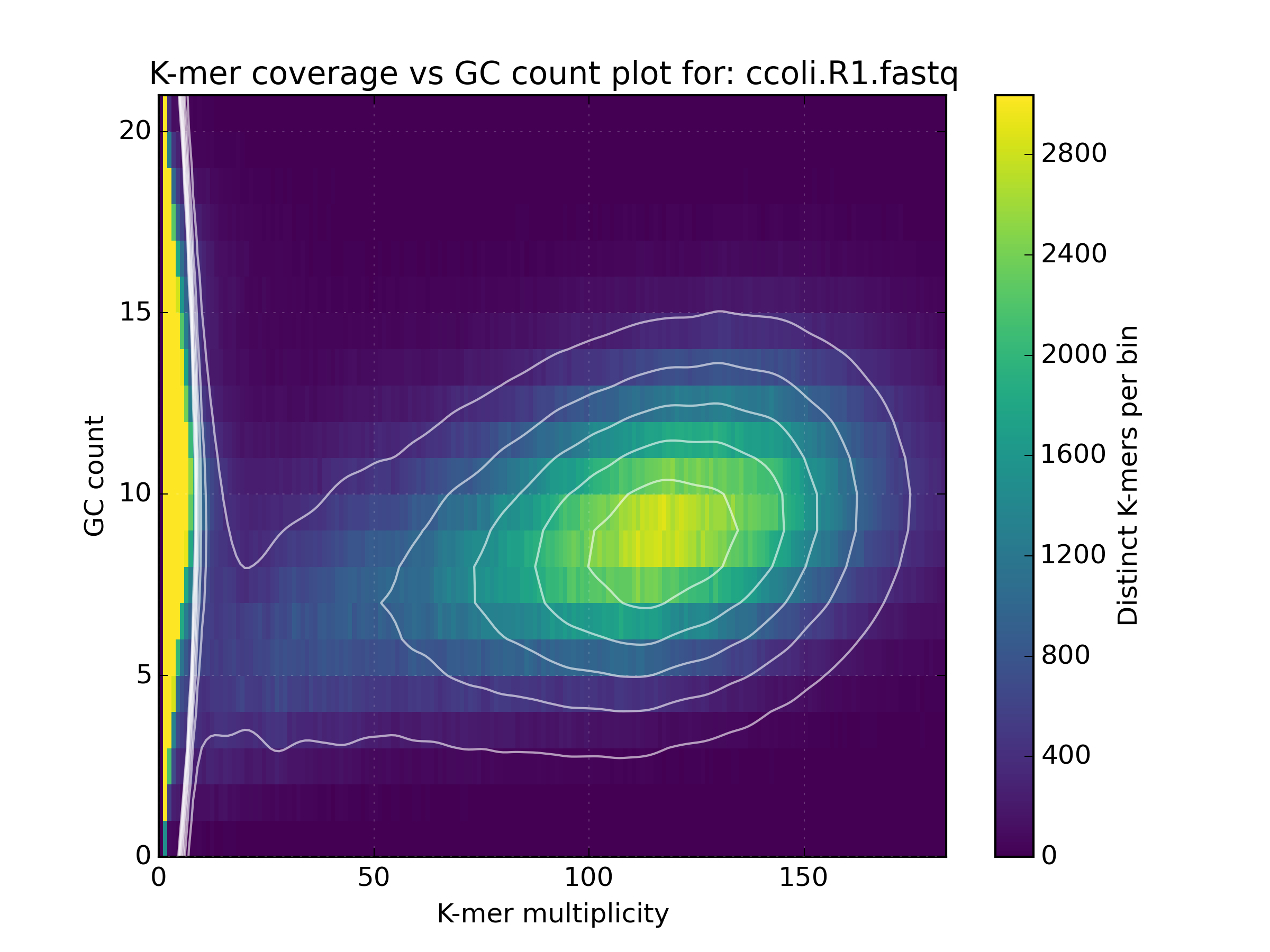
2.2. GCP
This tool takes in either a single jellyfish hash or one or more FastA or FastQ input files and then counts the GC nucleotides for each distinct K-mer in the hash. For each GC count and K-mer coverage level, the number of distinct K-mers are counted and stored in a matrix. This matrix can be used in much that same way as a kmer spectra histogram, although it provides richer output by incorperating GC content into the picture. This helps to distinguish legitimate content from contamination, which often appear as separate spots at unexpected GC and coverage levels.
Basic usage:
kat gcp (<input>)+
Output:
Produces a matrix file and associated Density plot. The matrix file starts with a header describing settings used to generate the matrix. Each header line starts with a ‘#’ character. The matrix that follows contains a space separated list of distinct k-mer counts for the GC-count indexed by the row. Each column index represents the K-mer Frequency. For example:
# Title:K-mer coverage vs GC count plot for: ERR409722_1.fastq ERR409722_2.fastq
# XLabel:K-mer multiplicity
# YLabel:GC count
# ZLabel:Distinct K-mers per bin
# Columns:1001
# Rows:27
# MaxVal:7705834
# Transpose:0
###
0 65392 10715 6038 4615 3769 3140 2690 2133 1748 1519 1370 1098 840 ...
0 189337 30772 20040 16630 15579 13673 12809 11890 10380 9605 8403 7370 6302 ...
0 428150 66753 41453 37478 34599 34622 34572 32740 31487 30356 28369 26880 ...
...
Applications:
- Assess data quality: estimates of kmers deriving from errors; sequencing bias
- Determine completeness of sequencing
- Identify genomic properties: Heterozygosity, homozygosity, karyotype, repeat content.
- Contamination detection
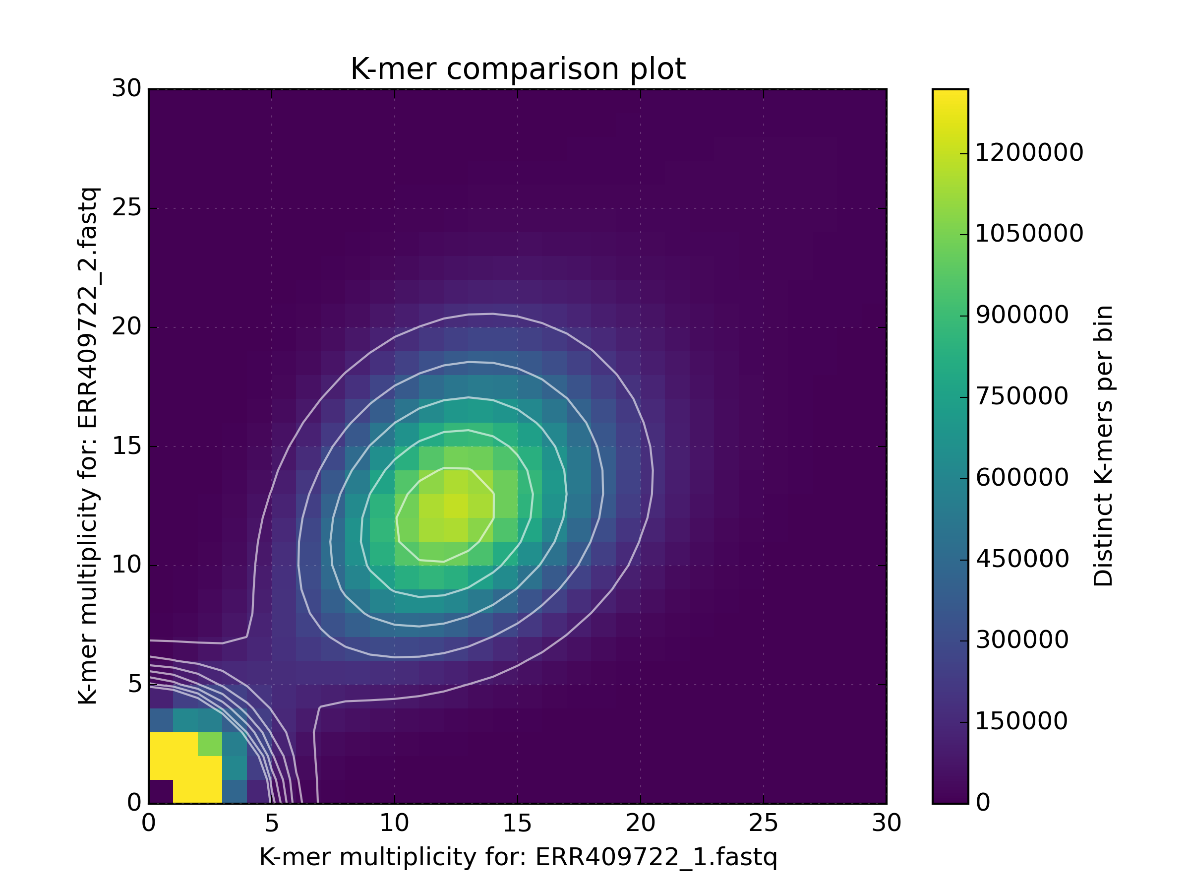
2.3. Comp
Compares jellyfish K-mer count hashes.
The most common use case for this tool is to compare two (or three) K-mer hashes. The typical use case for this tool is to compare K-mers from two K-mer hashes both representing K-mer counts for reads. However, it is also common to compare K-mers generated from reads to those generated from an assembly. If comparing K-mers from reads to K-mers from an assembly, the larger (most likely the read) K-mer hash should be provided first, then the assembly second. The third optional input acts as a filter, restricting the analysis to the K-mers present on that set. The manual contains more details on specific use cases.
Basic usage:
kat comp [options] <input_1> <input_2> [<input_3>]
Should the user wish to group multiple files to be concatenated into a single input group they may do so by surrounding the input group in single quotes. The following example groups the full input read set into the first input and compares against an assembly:
kat comp -t 8 -o pe_v_asm_test 'PE1.R1.fq PE1.R2.fq' asm.fa
… or more compactly:
kat comp -t 8 -o pe_v_asm_test 'PE1.R?.fq' asm.fa
… or if the reads are gzipped:
kat comp -t 8 -o pe_v_asm_test <(gunzip -c 'PE1.R?.fq') asm.fa
Output:
Produces a matrix file and by default a Spectra CN plot, although can also produce a Density plot if requested. The matrix file is structured in a similar way to the GCP tool with a header describing settings used to generate the matrix. Each header line starts with a ‘#’ character. The matrix that follows contains a space separated list of distinct k-mer counts for the frequency in each input file represented by the row and column index. For example:
# Title:K-mer comparison plot
# XLabel:K-mer multiplicity for: ERR409722_1.fastq
# YLabel:K-mer multiplicity for: ERR409722_2.fastq
# ZLabel:Distinct K-mers per bin
# Columns:1001
# Rows:1001
# MaxVal:57106148
# Transpose:1
###
0 57106148 2133673 428934 134189 45267 16399 6603 3374 2066 1371 930 752 490 ...
50919938 10364720 1613532 607932 239439 89985 36398 16589 8811 5469 3369 ...
1990321 1605550 1061952 561999 271443 125163 61769 34379 22459 15647 11171 ...
...
Applications:
- Determine sequencing bias between left and right read pairs.
- Compare the kmer spectrum of input reads against an assembly to gauge assembly completeness.
2.4. SECT
Estimates coverage levels across sequences in the provided input sequence file. This tool will produce a FastA style representation of the input sequence file containing K-mer coverage counts mapped across each sequence separated by spaces. K-mer coverage is determined from the provided counts input file, which can be either one jellyfish hash, or one or more FastA / FastQ files. In addition, a file containing statistics about each target sequence is produced.
NOTE: K-mers containing any Ns derived from sequences in the sequence file not be included.
Basic usage:
kat sect [options] <sequence_file> (<input>)+
Output:
Produces a FastA-style representation of the K-mer frequency across each target sequence as well as a file describing statistics for each target sequence. The FastA-style output might look like this:
>Chr4
31 31 31 29 29 29 28 27 27 28 28 28 30 30 30 29 29 29 29 31 32 32 33 33 33 31 29 30 ...
With an associated tab separated stats file which looks like this:
seq_name median       mean      gc%  seq_length  kmers_in_seq  invalid_kmers  %_invalid  non_zero_kmers  %_non_zero  %_non_zero_corrected
Chr4         26  362.45141  0.36204    18585056      18585036           3214    0.01729        18549840    99.81065              99.82792
- The column headers have the following meaning:
- seq_name - The name of the FastA/Q sequence
- median - The median K-mer coverage across the sequence
- mean - The mean K-mer coverage across the sequence
- gc% - The GC% of the sequence
- seq_length - The length of the sequence
- kmers_in_seq - The number of K-mers in the sequence. i.e. seq_length - K + 1
- invalid_kmers - The number of K-mers in the sequence that cannot be counted, most likely due to being non-canonical. i.e. non A,T,G,C
- %_invalid - The percentage of the sequence which contains invalid K-mers
- non_zero_kmers - The number of K-mers that have a coverage of 1 or greater
- %_non_zero - The percentage of the sequence which has a K-mer coverage greater than 1
- %_non_zero_corrected - The percentage of the sequence which has a K-mer coverage greater than 1 but ignoring any parts of the sequence represented by invalid K-mers.
Applications:
- Analyse K-mer coverage across assembled sequences
- Compare assemblies using K-mers, helpful to levels of contamination of a specific organism.
- Contamination detection - Compare K-mer spectrum against assembly providing average coverage and GC values for each contig, which can be 2D binned and plot as a heatmap
2.5. Filtering tools
KAT comes with two filtering tools allowing the user to slice and dice their data in a rapid and simple way.
2.5.1. K-mer filtering
This tool allows the user to produce K-mer hashes, within and outside user defined GC and k-mer coverage bounds. This is useful for isolating k-mers that could be attributable to contamination, or for contamination removal. Normally, the user would identify such regions using plots from the GCP tool.
Basic usage:
kat filter kmer [options] (<input>)+
Applications:
- Extracting k-mers with defined GC and coverage
- Contamination extraction (from k-mer hash)
2.5.2. Sequence filtering
The user loads a k-mer hash and then filters sequences (either in or out) depending on whether those sequences contain the k-mer or not. The user can also apply a threshold requiring X% of k-mers to be in the sequence before filtering is applied. The user can also use this tool for filtering paired end reads, and for subsampling.
Basic usage:
kat filter seq [options] --seq <seq_file> <k-mer_hash>
Applications:
- Contamination extraction from read file or assembly files, extraction of organelles, subsampling high_coverage regions
2.6. Plotting tools
KAT comes with a selection of plotting tools for representing and comparing K-mer spectra in various ways. All plotting tools come with the ability to manually modify axis, titles, limits, size, resolution, etc, although they will all try to pick intelligent defaults directly from the data provided.
2.6.1. Spectra hist
Visualises the K-mer spectra from kat hist or jellyfish histo output.
This tool is designed to plot line graphs of one or more histograms. The idea is
to be able to compare total K-mer counts between different datasets.
Basic usage:
kat plot spectra-hist <hist_file>
Applications:
- Basic K-mer spectra visualisation
2.6.2. Density
Creates a scatter plot, where the density or “heat” at each point represents the
number of distinct K-mers at that point. Typically this is used to visualise a
matrix produced by the kat comp tool to compare frequencies from two K-mer
hashes produced by different NGS reads, or to visualise the GC vs K-mer matrices
produced by the kat gcp tool.
Basic usage:
kat plot density <matrix_file>
Applications:
- Visualise GC vs coverage matrices
- Visualise coverage vs coverage matrices
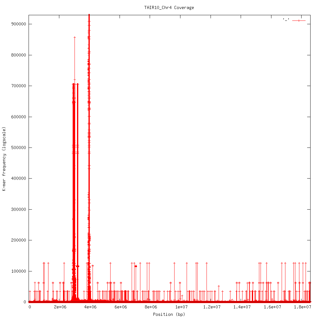
2.6.3. Profile
Shows K-mer coverage level across an sequence
Basic usage:
kat plot profile <sect_counts_file>
Applications:
- Visualise coverage (and optionally GC) levels across a sequence or set of sequences
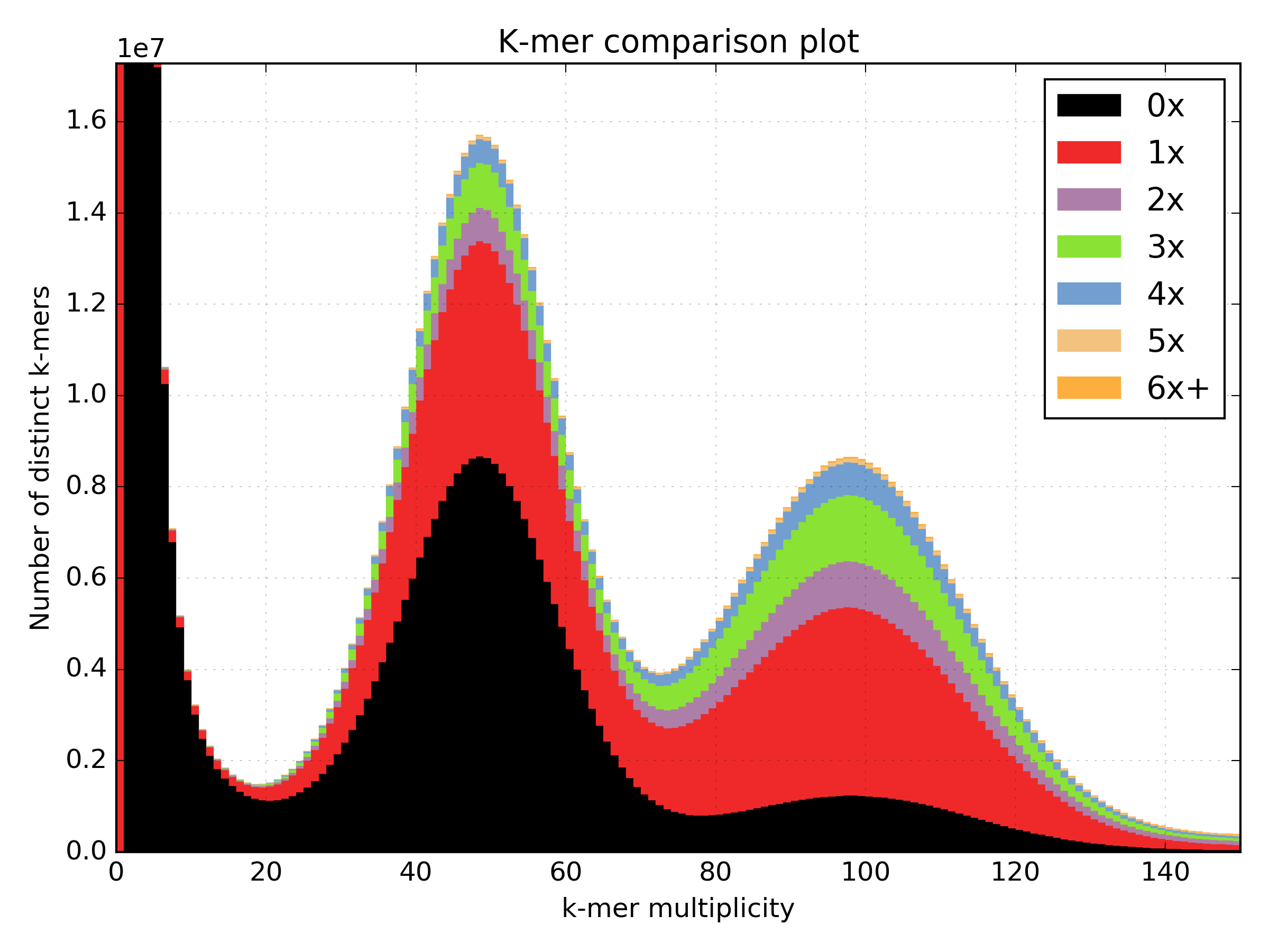
2.6.4. Spectra CN
Shows K-mer duplication levels, which correspond to copy number variation within
an assembly by comparing K-mers found in sequenced reads, to K-mers found in an
assembly of those reads. Uses matrix output from the kat comp tool.
Basic usage:
kat plot spectra-cn <matrix_file>
Applications:
- Visualise the copy number spectra of WGS data compared against an assembly
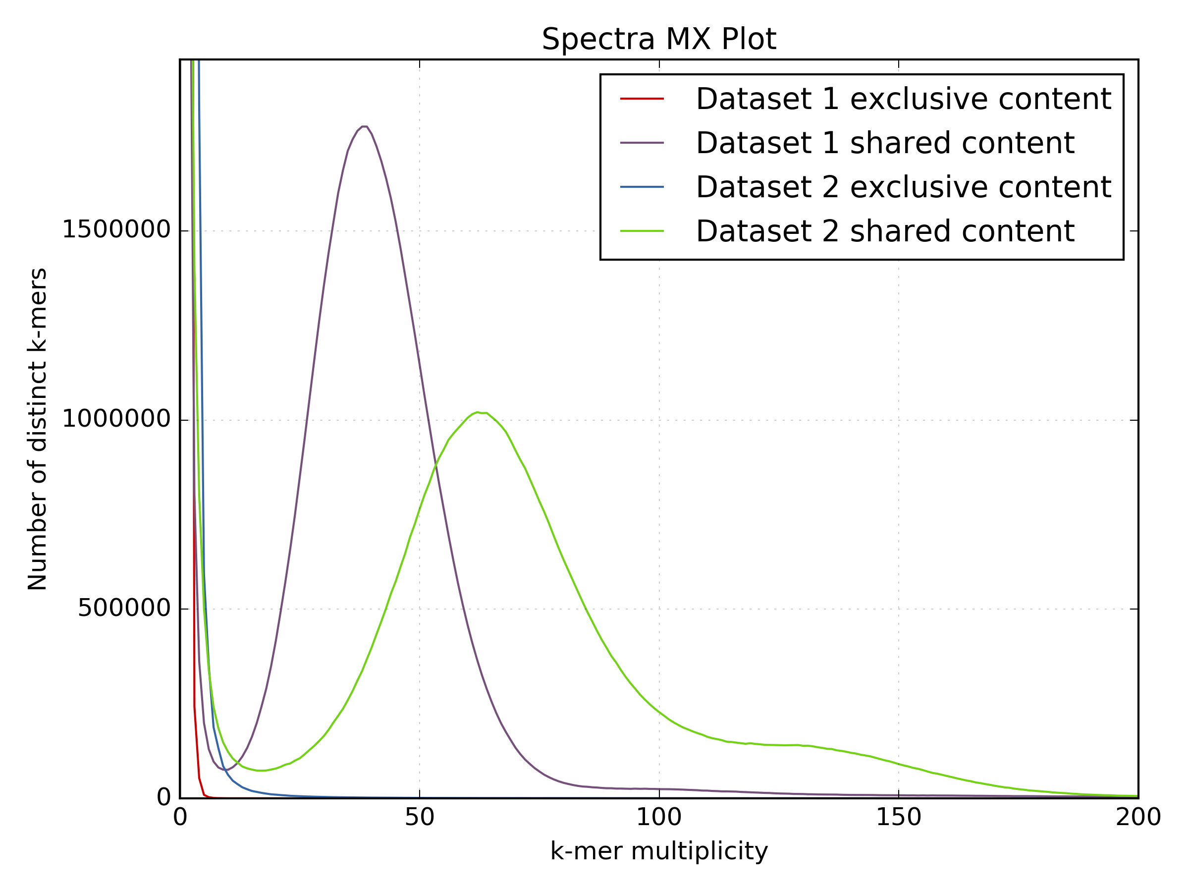
2.6.5. Spectra MX
Produces K-mer spectras from rows or columns in a matrix generated by kat comp.
This tool is designed to plot line graphs for one or more histograms, each histogram
being represented by a single row or column in the matrix.
This tool also has a special mode for showing shared and exclusive content between
two different samples. This mode takes the first row and column of the matrix representing
content which is found exclusively in each sample. Two more lines are plotting,
one which has each following row summed, and the other that has each following column
summed. These two plots represent the shared content for each sample. This mode
can be activated using the --intersection flag.
Alternatively, you can select specific rows and columns from the matrix using a
comma separated list identified with the --list option. Each element in the
list should start with either a ‘c’ or a ‘r’ indicating whether or not the column
or row is requested. Then the element should contain a number indicating which
column or row to select. For example: --list c0,r1 will select column 0 and
row 1. Note: spaces are not tolerated in this list.
Basic usage:
kat plot spectra-mx <matrix_file>
Applications:
- Visualising shared and exclusive content between two datasets
- RNAseq to WGS comparison
- Visualising k-mer spectra of arbitrary columns and rows from a matrix